 Documentation
Interactive Counting
Documentation
Interactive Counting
Interactive Density Counting
Overview, what it can and cannot do
The purpose of this workflow is to enable counting of objects in crowded scenes such as cells in microscopy images. Counting is performed by directly estimating the density of objects in the image without performing segmentation or object detection.
When the density of objects in the image is low and the objects are well separated from each other, it is possible to count objects by first segmenting the foreground and then collecting the connected components as it is done in the Object Classification workflow. However, as the density of the objects increases, the latter approach underestimates the number of objects due to under-segmentation errors.
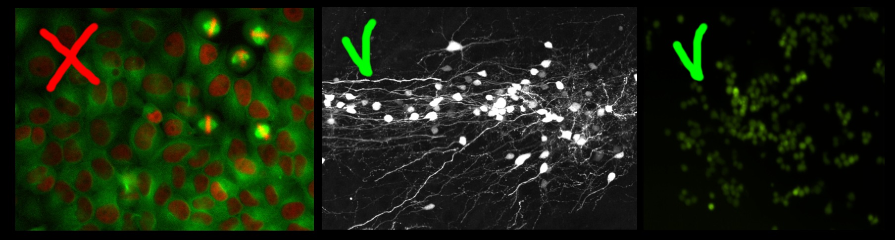
This workflow offers a supervised learning strategy to object counting that is robust to overlapping instances. It is appropriate for counting many blob-like overlapping objects with similar appearance (size, intensity, texture, etc..) that may overlap in the image plane. Let’s discuss three examples.
The left image in the figure below contains large non-overlapping objects with high variability in size and appearance (red nuclei and mitotic yellow nuclei) . Therefore it is best suited for the Object Classification workflow. The two right images in the figure below contain small overlapping objects that are difficult to segment individually. The objects in each of these images have similar appearance and similar same size, therefore these two images are appropriate for the Density Counting workflow.
This workflow will estimate directly the density of objects in the image and infer the number of objects without requiring segmentation.
How does it work, what should you annotate
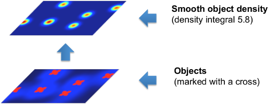
In order to avoid the difficult task of segmenting each object individually, this workflow implements a supervised object counting strategy called density counting. The algorithm learns from the user annotations a real valued object density. Integrating over a sufficiently large image region yields an estimate of the number of objects in that region. The density is approximated by a normalized Gaussian function placed on the center of each object.
In the following figure, note that the integral of the smooth density is a real number close to the true number of cells in the image.
It is important to note that the object density is an approximate estimator of the true integer count. The estimates are close to the true count when integrated over sufficiently large regions of the image and when enough training data is provided.
NOTE that also contaminations of the image such as debris or other spurious objects may invalidate the estimated density.
Please refer to the references for further details.
The user gives annotations (see tutorial below) in the form of dots (red) for the object centers and brush-strokes (green) for the irrelevant background. A pixel-wise mapping between local features and the object density is learned directly from these annotations.
This workflow offers the possibility to interactively refine the learned density by:
- placing more annotations for the foreground and background
- monitoring the object counts over sub-image regions
Interactive Counting Tutorial
Let’s warm up with a small tutorial.
1. Input Data
Similarly to other ilastik workflows, you can provide either images (e.g. *.png, *.jpg and *.tif) directly or pass hdf5 datasets. The image import procedure is detailed in Data Selection. Please note that the current version of the Counting module is limited to handling 2D data only, for this reason hdf5-datasets with a z-axis or a temporal axis will not be accepted. Only the training images required for the manual labeling have to be added in this way, the full prediction on a large dataset can be done via Batch Processing Data Selection. In the following tutorial we will use a dataset of microscopic cell images generated with SIMCEP. This dataset is publicly available at the following link.
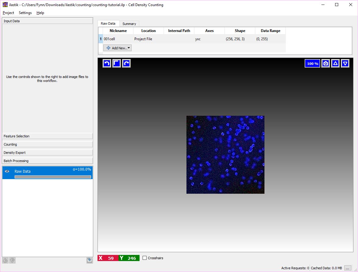
In this tutorial we have already imported an image in the project file counting-tutorial.ilp.
As a first step, let us just load this project. You should be able to start from the window below.
2. Feature Selection
The second step is to define some features. Feature selection is similar to the Pixel Classification Workflow.
The image below shows an example of feature selection. In particular, blob-detectors like the Laplacian of Gaussians or line-detectors like the Hessian of Gaussians are appropriate for blob like structure such as cells. The figure below shows the response of the Laplacian of Gaussians filter.
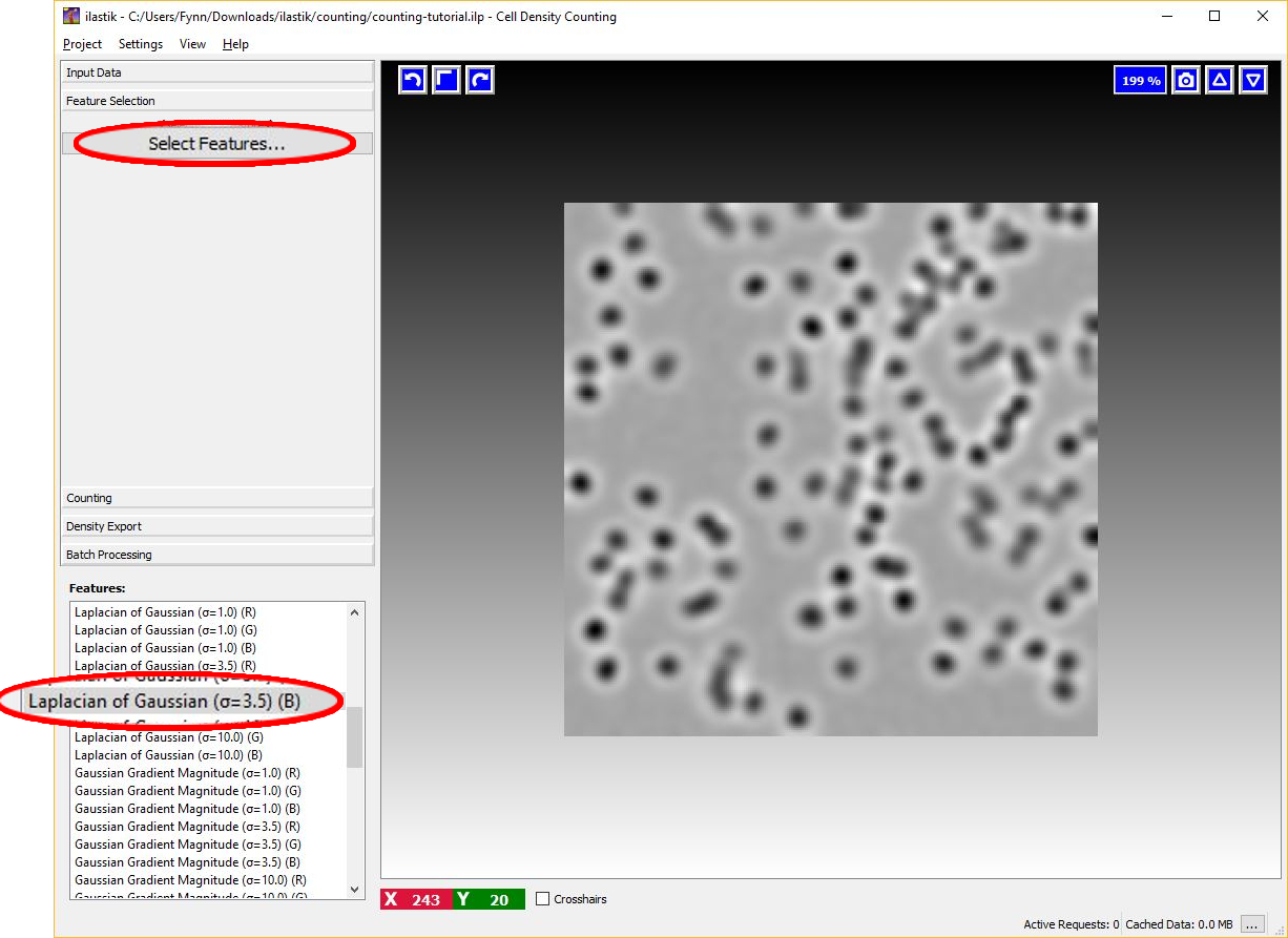
It is appropriate to match the size of the object and of the cluster of objects with the scale of the features as shown in the figure below. For further details on feature selection please refer to How to select good features.

3. Interactive counting
Annotations are done by painting while looking at the raw data and at the intermediate results of the algorithm. The result of this algorithm can be interactively refined while being in Live-Update mode. The overall workflow resembles the Pixel Classification Workflow. The main difference is that the Density Counting workflow gives the user the possibility to:
- add dots for the object instances (see tips below)
- add brush strokes over the background
- add boxes to monitor the count in sub-image regions.
These list of interactions is typically performed in sequence. This idea is reflected in the layout of the left control panel that is typically used from top to bottom.
3.1 Dotting
This is the first interaction with the core of this workflow. The purpose of this interaction is to provide the classifier with training examples for the object centers and training examples for the background.
To begin placing dot annotation select the red Foreground label and then on click on the image. The annotation has to be placed close to the center of an object (cell) as in the figure below.
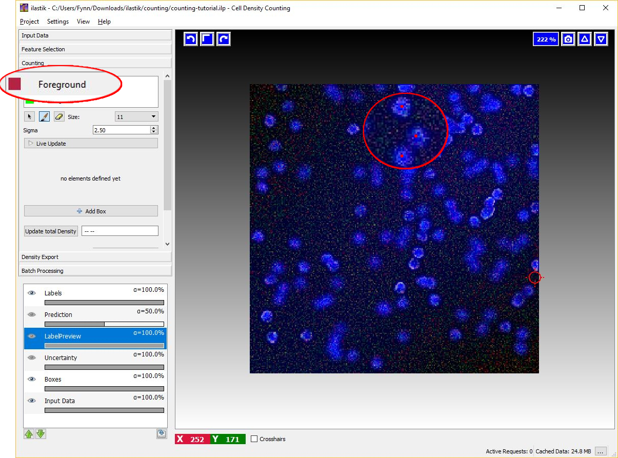
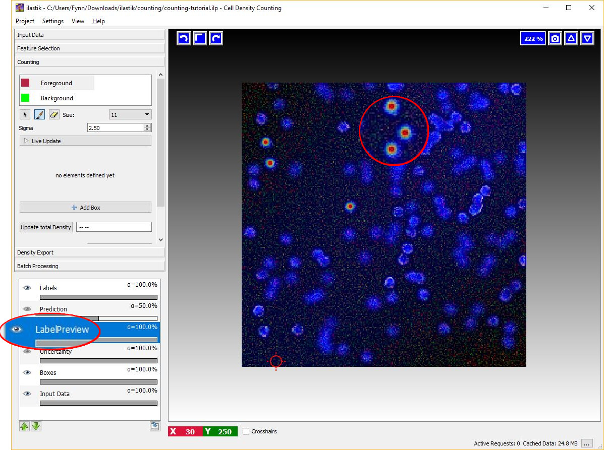
Given the dotted annotations, a smooth training density is computed by placing a normalized Gaussian function centered at the location of each dot. The scale of the Gaussian is a user parameter Sigma which should roughly match the object size. To help deciding an appropriate value for this parameter you will see the that the size of the crosshair-cursor changes accordingly to the chosen sigma (in the left panel). In addition, the density which is used during training is saved in the LabelPreview layer as shown in the figure below.
Different choices for the parameter Sigma are shown below. On the left image, the value of sigma is chose too small, while on the right the value of sigma is too large. The center image shows a well chosen sigma.
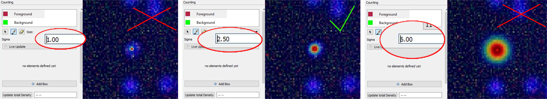
NOTE: Large values for sigma can impact the required computation time: consider using a different counting approach, such as the Object Classification workflow if this parameter has to be chosen larger than 5.
3.2 Brushing
After a few dots have been placed (say around 10 - 20 depending on the data) we can add training examples for the background.
Background labeling works the same as in the Pixel Classification Workflow.
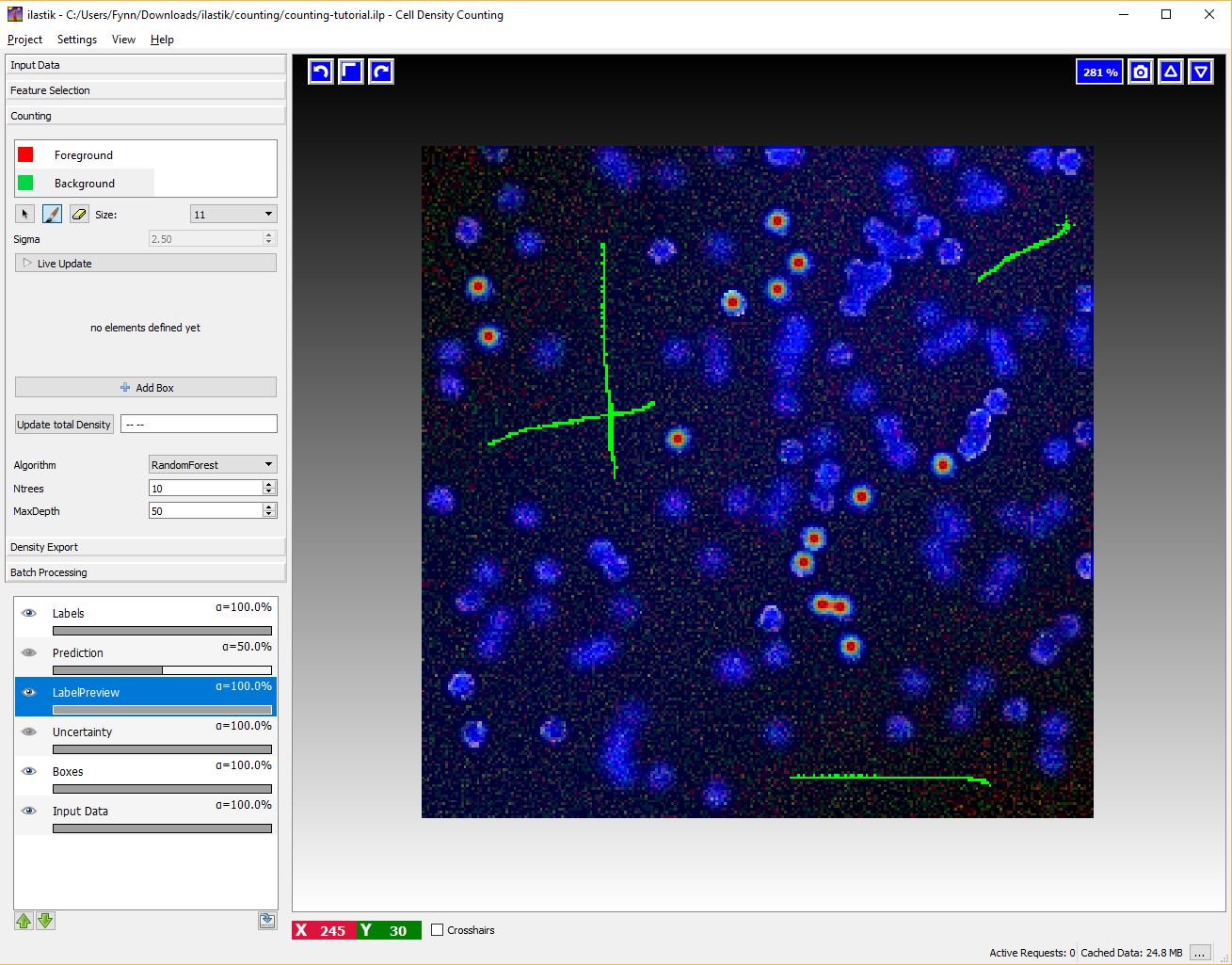
To activate this interaction select the green Background label and give broad strokes on the image, as in the figure below, marking unimportant areas or regions where the predicted density should be 0.
4 Live Update Mode
After some labels for the objects and the background have been given, switch the Live-Update on (using the Live Update button), this will trigger a first prediction, displayed in the Prediction-Layer.
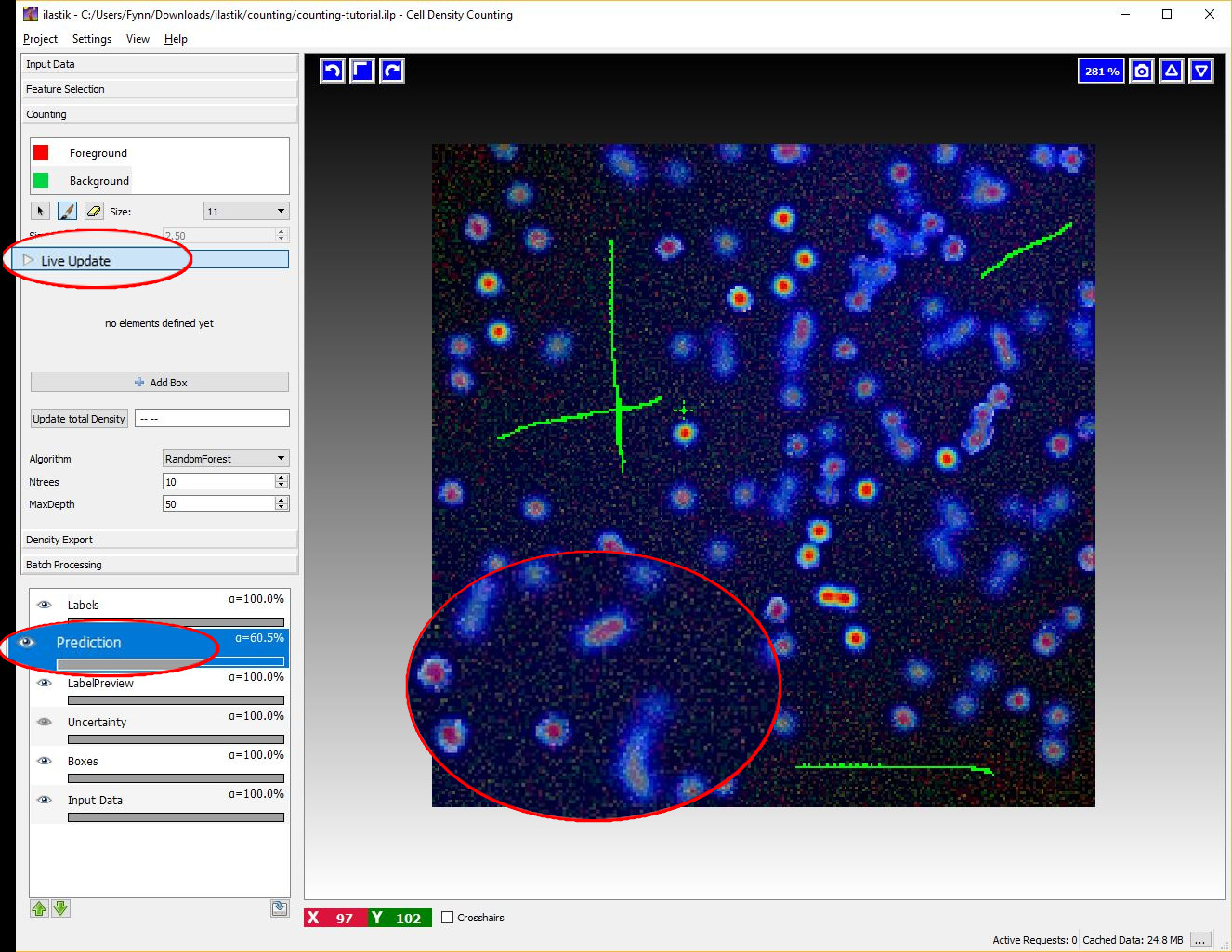
If the Live Update Mode is active, every single change in the training data (e.g. placing new labels or changing parameters) causes a new prediction - thus it may be faster to toggle it OFF again when you plan extensive modifications.
How do we get from the density to the number of objects?
This is explained in the next section.
5 Box Interaction Mode
This interaction takes place after we have pressed the Live Update Button for the first time. The boxes are operator windows that integrate the density over a certain image region. Therefore they provide the predicted counts for the objects in that region.
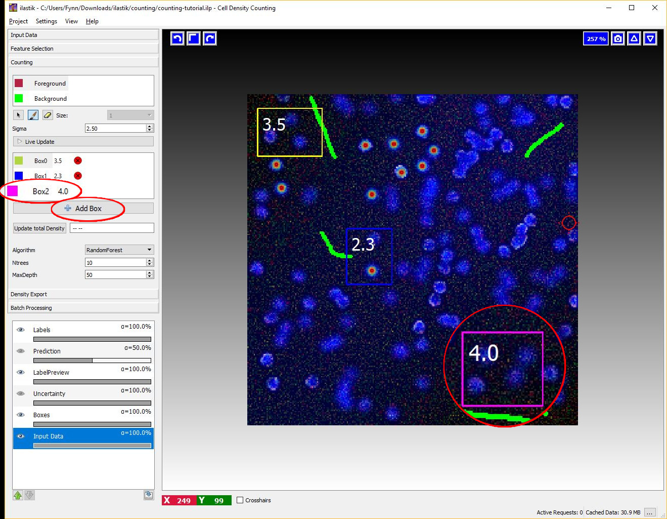
You can start placing boxes by selecting the Add Box button and drawing a rectangular region on the image from the top left to the bottom right. The new box will be added automatically to the Box List. Boxes show the object count for the region on the upper right corner and beside the box name in the Box List as it is shown in the next figure.
Boxes can be:
-
Selected and Moved: to select a particular you can select its name the Box List or just pass over it with your mouse. Note that when you pass over a particular box with the mouse, its name in the BoxList is highlighted. The box will change color once selected. You can now drag the box in a different position by clicking and moving the mouse while pressing the
Ctrlkey. -
Resized: when selecting a box it will show 2 resize handles at its right and bottom borders.
-
Deleted: to delete a box either click on the delete button (a red cross) on the BoxList or press
Delwhile selecting the box -
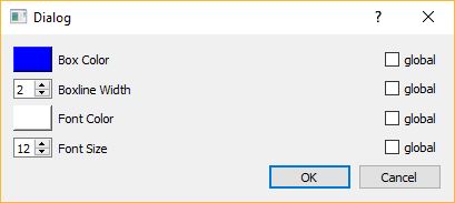
Configured: you can configure the appearance (color, fontsize, fontcolor etc…) of each individual box (or of all boxes at the same time), by double-clicking on the colored rectangle in the BoxList. The interaction dialog for the box properties is shown below.
You can continue adding boxes and provide new annotations (dots or brushes) for object centers and background until you are satisfied of the counting results as shown by the boxes.
6 Counting the entire image
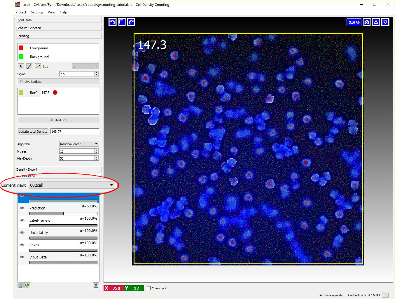
Let us switch to another image by using the Current View menu on the left (Note that this is only available, if more than one dataset is loaded into the project). As is shown in the image below, this image is free from annotations and the prediction of the density is not yet computed. However, the algorithm is already trained and therefore we are ready to compute the density for this new image. As before, it is possible to start the prediction by toggling the Live Update button and monitor the results with a box. However, let us press the Update total density button on the left. This button estimates the predicted count for the entire image.
If the training labels are sufficient, we should obtain a count similar to what is shown in the image below that matches the number of objects in the images.
Note: In a real world scenario, you may need to distribute several annotations across many images to obtain accurate counts for all the images in the dataset.
You are now ready to use the workflow on your data! Please continue to read if you want to know some advanced features.
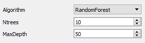
The Algorithm
Random Forest
This approach uses a Random Regression Forest as regression algorithm.
The implementation of the random regression forest is based on sklearn.
Advanced parameters
The forest parameters exposed to the user are:
- Ntrees number of trees in the forest
- MaxDepth maximum depth of each individual tree.
Both of these parameters influence the smoothness of the prediction and may affect performance. On the one side, too few and too shallow trees can cause under-fitting of the density. On the other side, too many and too deep trees may also lower performance due to over-fitting and slow down the algorithm computation. This workflow gives the user the possibility to manually tune these parameters.
4. Exporting results
We can export the results for all the images that were added to the project. This processing follows a standard ilastik procedure that is demonstrated here.
5. Batch Processing unseen images
For large-scale prediction of unseen images, the procedure is to first interactively train the regressors on a representative subset of the images. Then, use batch processing for the rest of the data. The batch processing follows a standard ilastik procedure that is demonstrated here.
This workflow supports the hdf5 format to store the density for the batch processed images. The density for the batch processed image is stored as a dataset of the hdf5 file, which is easily readable with Matlab or Python. The density can then be integrated to retrieve the count of objects in the image.
NOTE: the density can be exported also as a normal grayscale image (*.png, *.tiff, etc..). However, due to normalization, the intensity value of the image do not correspond anymore to the predicted density values (originally between 0,1).
6. References
[1] L Fiaschi, R. Nair, U. Koethe and F. A. Hamprecht. Learning to Count with Regression Forest and Structured Labels. Proceedings of the International Conference on Pattern Recognition (ICPR 2012), Tsukuba, Japan, November, 2012.